Data & Simulation / A Build Log

From Zero to MATLAB:
When an AI Learned to Engineer

A single-session chronicle of connecting Claude Desktop to MATLAB, crossing five setup walls, and building five simulations that model the physical world.

By T Pavan Kumar · Illustrated with data from the session on March 25, 2026

Interface

Claude Desktop

Natural-language prompts

→

Bridge

MATLAB MCP Server

Tool discovery and code execution

→

Runtime

MATLAB R2025b
+ Simulink

Windows 11, trial license

The architecture: a natural-language interface controlling professional engineering software.

The assignment looked like a ten-minute integration: connect Claude Desktop to MATLAB, ask a question, and watch the tools light up. Instead it became an afternoon of licensing dead ends, installation traps, a hard reset, one crucial runtime lesson, and five experiments that escalated from a single sine wave to a deep fractal zoom.

This merged version keeps both original tellings in one place. It preserves the build-log narrative from the setup session and the quantitative record of what happened once the bridge existed.

Chapter I

The Assignment and First Contact

The directive came from Anand during a conversation about AI tools and professional software. The pattern was already established: Claude had been connected to Blender for 3D modeling and to ROS for robotics. The next question was whether that same pattern could stretch into engineering and mathematical computation through Claude Desktop.

"We are creating a series of environments, not just coding environments but other kinds of software, and seeing how coding agents can work with them."

— Anand S, during the initial briefing

Two directions were clear from the start. One was about making things easier: describe an engineering problem in plain English and let Claude assemble the solution. The other was about discovering new possibilities: use Claude Desktop to explore design spaces, generate novel simulations, and push toward results that would not have emerged from a static prompt alone.

The starting point was simple on paper: find an MCP server for MATLAB, or build one. The first discovery was encouraging. MathWorks had already published an official open-source MATLAB MCP Core Server on GitHub. The session notes record 269 stars, active development, a fresh v0.6.1 release, a Go-based binary distribution, and a .mcpb bundle designed to install into Claude Desktop with a double-click. The infrastructure, it seemed, was ready.

When the connection finally came alive, the very first question was the most basic one: What do I actually have to work with? The answer was stark. detect_matlab_toolboxes revealed MATLAB R2025b and Simulink, and nothing beyond that. No Control System Toolbox. No Signal Processing Toolbox. Just the raw engines. That constraint became the story, because every experiment that followed had to be built from first principles.

Discovery

What Was Available vs. What Was Needed

Toolboxes Found

Specialty Toolboxes

MCP Tools Available

Simulations Built

detect_toolboxes

✓ Used

evaluate_code

Primary

run_matlab_file

Available

check_code

Available

run_test_file

Available

Only two of the five available MCP tools ended up carrying the whole session: toolbox discovery and live code evaluation.

Chapter II

Five Walls Before the First Tool Call

What followed was not a demo reel. It was a debugging sequence: five distinct blockers, a different fix for each one, and the kind of setup narrative that usually disappears from polished product stories even though it defines the real experience of working with new tools.

Licensing Error 9 MATLAB refused to start because the license was bound to a different Windows username. The active user, admin, was not authorized.

Missing Activation Tool The standard fix failed because activate_matlab.exe was missing from the expected path.

No License Linked The MathWorks License Center reported another dead end: the account was not currently linked to any licenses.

FIX

The Nuclear Option The recovery path was a full uninstall and a fresh MATLAB R2025b install with a new trial license activated under the correct username.

The .mcpb Bundle Did Not Install Cleanly The promised double-click flow stalled, so the server had to be installed manually through Claude Desktop settings.

MCP Could Not See MATLAB MATLAB worked from the command line, but the MCP server still reported no installation because the PATH change had to live in the System PATH and be propagated into the server context.

The fixes were all different. The licensing issue demanded a reinstall. The discovery issue demanded a System PATH update rather than a User PATH edit. The bundle issue demanded a manual install route through Claude Desktop. Each wall fell in a different way, and each fix only became real after everything was restarted and tested again.

Claude Desktop · MATLAB MCP

User: What MATLAB toolboxes do I have installed?

Claude: -> detect_matlab_toolboxes

MATLAB 25.2 (R2025b)
Simulink 25.2 (R2025b)
No additional specialty toolboxes detected.

Running on Windows 11 Pro with a trial license.

That first successful tool call changed the shape of the session. The problem was no longer whether Claude could see MATLAB. The problem became whether it could do serious engineering work with only core MATLAB, Simulink, and one active conversational thread.

III

Chapter III

Five Simulations, One Thread

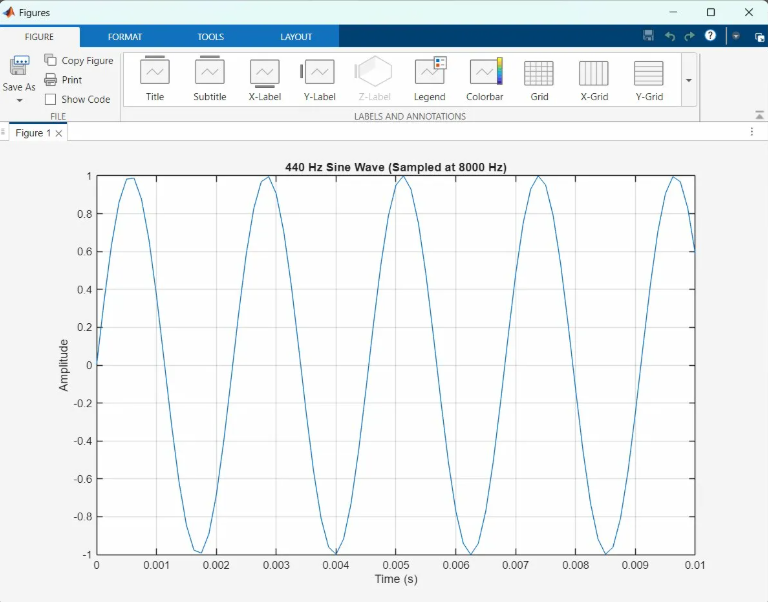
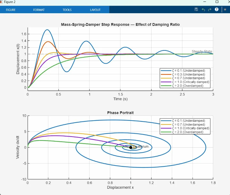
The experiment sequence followed a clear arc. Each simulation built on the intuition of the one before it: start with a single oscillation, move into classical mechanics, add coupled dynamics, step into closed-loop control, and finish with a piece of pure mathematical exploration.

Session Arc

From First Signal to Deep Zoom

Simulation 01

440 Hz Sine Wave

A concert-pitch A note sampled at 8,000 points. The simplest possible proof that the bridge was real, and the moment a figure window first appeared on the desktop.

✓ Clean run Analytical

Simulation 02

Mass-Spring-Damper

A single-DOF oscillator with five damping ratios, from ζ = 0.1 to 2.0. The prompt asked for three cases; Claude delivered five plus phase portraits that showed spiral and direct approaches to equilibrium.

✓ Clean run Analytical

Simulation 03

Quarter-Car Suspension

A two-DOF RK4 model sweeping four suspension configurations over an 8 cm speed bump at 30 km/h. One sentence unfolded into body response, ride comfort, suspension travel, tire deflection, and a normalized trade-off comparison.

✓ Clean run Numerical

Simulation 04

Simulink PID Controller

A programmatically built control loop with a step source, sum junction, PID block, plant, and feedback path. Five tuning strategies were simulated, compared, and turned into step response, tracking error, control effort, and metrics views.

✗ Failed once ✓ Fixed and run

Simulation 05

Mandelbrot Deep Zoom

Three rendering passes: the full set at 1600 × 1200, Seahorse Valley at 87× zoom, and a mini-Mandelbrot exploration at 350×. The narrative notes compress that visual journey into a roughly 90× deep zoom into a self-similar copy.

✓ Clean run 5.28M pixels

Total MCP Calls

83%

First-Run Success

Failure Resolved

5.4M

Data Points Generated

"The first run failed. That single error taught more about the platform's constraints than any documentation could."

Chapter IV

Five Prompts, Five Worlds

What followed was a rapid escalation. Each prompt was about a sentence long. Each result was a full analysis that would normally take thirty minutes to an hour to code by hand, yet the session was driven entirely through Claude Desktop and the MATLAB bridge.

Demos Created

Sentence Each

Lines Written by Hand

Experiment 01

440 Hz Sine Wave

✓ Clean run Signal proof

A 440 Hz signal sampled at 8,000 Hz became the first unmistakable proof that the connection was real. Claude wrote the MATLAB code, executed it, and the figure appeared on the desktop.

In the data-story framing, this was the simplest line of physics in the whole session: y = sin(2πft). In the build-log framing, it was the instant the bridge stopped being theoretical and started behaving like a tool.

1 DOF 8,000 samples 440 Hz Analytical

Sine wave MATLAB output plot — Placed image **Sine Wave Output**
The renamed `sine-wave.png` image matches the first proof-of-connection experiment.

Experiment 02

Mass-Spring-Damper with Phase Portrait

✓ Clean run Dynamics

The second experiment shifted from proof-of-connection to real dynamics. The prompt asked for three damping ratios; Claude returned five, spanning ζ = 0.1 to 2.0, and added a phase portrait without being explicitly asked.

That made the result more than a textbook curve family. It became an interpretive visualization of underdamped spirals, critical damping, and overdamped return to equilibrium, all derived analytically from a one-degree-of-freedom system.

1 DOF 15,000 data points 5 damping ratios Phase portrait

Mass spring damper plots and phase portrait — Placed image **Oscillator Plots**
The `mass-spring-damper.png` image fits the second dynamics experiment and its phase-space view.

Experiment 03

Quarter-Car Suspension Analysis

✓ Clean run Automotive

One sentence, "design a suspension system for a car hitting a speed bump," turned into a much richer engineering study. Claude built a two-degree-of-freedom quarter-car model, drove it over an 8 cm bump at 30 km/h, and compared four suspension configurations with RK4 integration.

The qualitative output was a six-panel analysis covering body response, ride comfort, suspension travel, tire deflection, and a normalized trade-off view. The quantitative record says the run produced 80,000 output points from 20,000 × 4 integration steps, and the session notes also describe the working version as computing roughly 5.3 million state updates.

2 DOF RK4 4 configs 80,000 outputs 5.3M state updates

Quarter car suspension analysis dashboard — Placed image **Suspension Dashboard**
The `car-suspension.png` image maps directly to the quarter-car study and multi-panel ride analysis.

Experiment 04

PID Controller with Simulink

✗ Failed once ✓ Fixed

This was the most architecturally ambitious build in the session. Claude assembled a Simulink feedback model programmatically with a step source, a summing junction, a PID block, a plant, and a feedback loop.

Once it ran cleanly, the model compared five tuning strategies and produced step responses, tracking-error curves, control-effort analysis, and a performance-metrics table. The quantitative summary records roughly 50,000 data points and an ode45-driven simulation path under the broader Simulink workflow.

Simulink 5 tunings ~50,000 points ode45

Simulink PID controller study output — Placed image **PID Control Study**
The `simulink.png` image belongs with the PID controller experiment built in Simulink.

Experiment 05

Mandelbrot Deep Zoom

✓ Clean run Fractal rendering

The final experiment moved from engineering simulation into exploratory mathematics. Claude rendered the full Mandelbrot set, identified Seahorse Valley as an interesting target, and then kept zooming toward a mini-Mandelbrot structure.

The data story breaks that output into three passes: the full set at 1600 × 1200, a Seahorse Valley view at 87×, and a deeper 350× exploration with custom pchip-interpolated colormaps and smooth iteration coloring to remove banding. The narrative account compresses the visual effect into a roughly 90× deep zoom and emphasizes that Claude knew where to zoom and how to reveal the structure.

2D grid 5.28M pixels 87x and 350x zooms Escape-time

Primary Mandelbrot fractal render — Placed image **Primary Fractal Render**
The wide `mandelbrot-fractal.png` image works as the main overview frame for the Mandelbrot section.

Mini Mandelbrot deep zoom render — Placed image **Mini-Mandelbrot Deep Zoom**
The `mini-mandelbrot.png` file is preserved as the second fractal image to show the deeper zoom target.

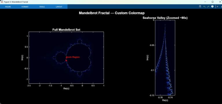
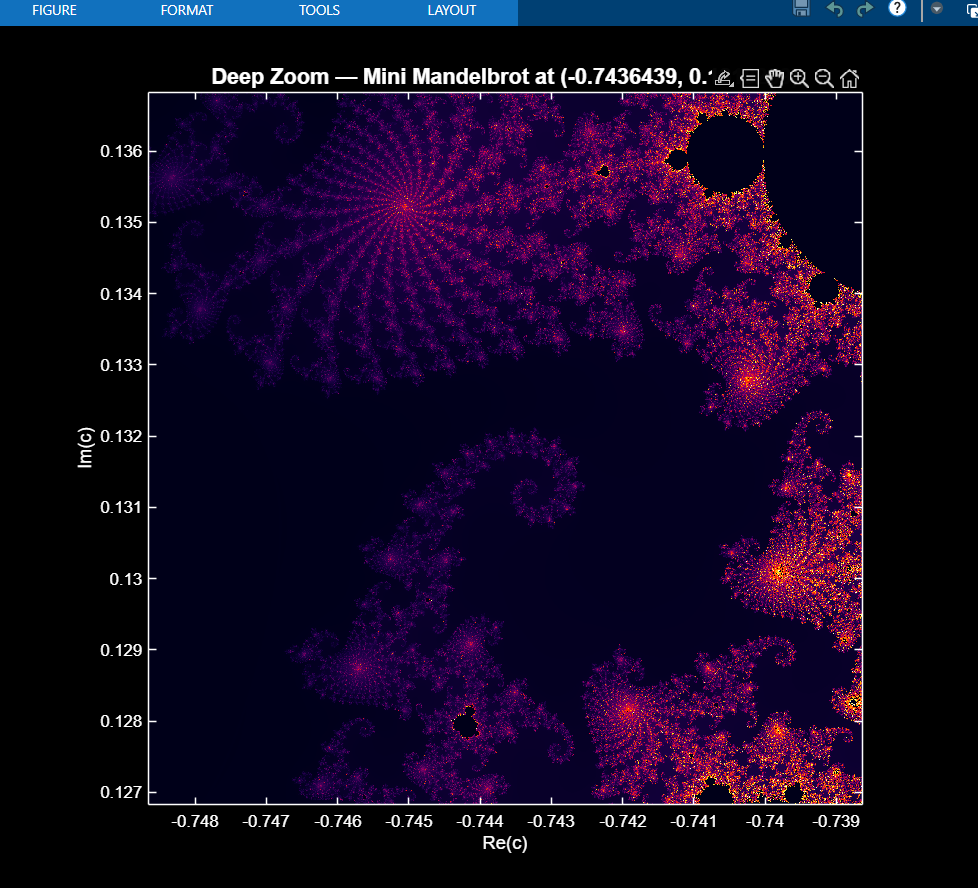
What started as a toolbox inventory ended with a Simulink model on disk and a fractal sequence that crossed 5.28 million rendered pixels. The session ran from the trivially analytical to the numerically intensive, then into control architecture, and finally into pure computation.

Chapter V

The Numbers and the Constraint

Each experiment pushed the computational footprint further: more state variables, more output, more iteration, and a wider spread between analytical and numerical methods. The quantitative summary from the second story is preserved below in full.

Quantitative Summary

Computational Footprint by Simulation

Simulation	DOF / Dims	Data Points	Iterations	Method	Outcome
Sine Wave	1	8,000	—	Analytical	Pass
Mass-Spring-Damper	1	15,000	—	Analytical	Pass
Quarter-Car	2	80,000	20,000 × 4	RK4	Pass
PID Controller	2+	~50,000	ode45	Simulink	Fail → Pass
Mandelbrot	2D grid	5,280,000	500-2,000	Escape-time	Pass

Scale

Computational Scale Across Simulations

Sine Wave

Spring-Damper

15K

Quarter-Car

80K

PID / Simulink

~50K

Mandelbrot

5.28M pixels

Not everything worked on the first try. The most important runtime lesson of the day was that evaluate_matlab_code behaves like script execution, not like running a saved function file. Helper functions defined at the end of the script with the usual function keyword were not reliably visible in that execution mode.

The fix was immediate and revealing: convert the helper logic into anonymous functions that live directly in the active workspace. Same mathematics, different packaging. That one change turned a failure into a clean run and mapped a real platform constraint that only surfaced because the code was being executed against a live system.

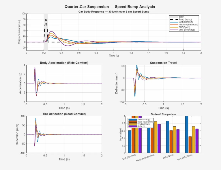
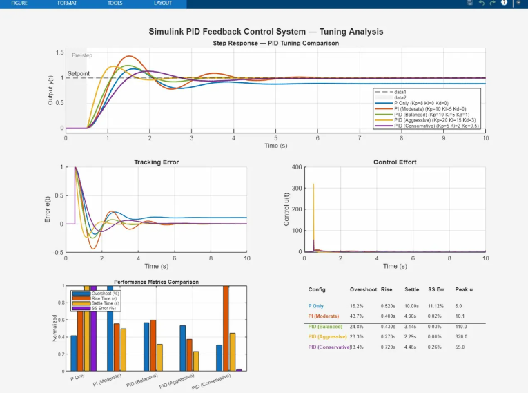
Session note reconciliation. The progression timeline marks the Simulink PID controller as the single failed-first-run experiment, while the preserved debugging example uses a qcar_dynamics helper from the suspension work. Both records are kept here because they point to the same practical lesson: under live evaluate_matlab_code execution, helper logic had to be rewritten as anonymous functions inside the active workspace.

Debugging

The Failure That Mapped the Constraints

✗ Attempt 1 — Failed

% Helper function at end of script
% MATLAB cannot find it during eval

for i = 1:N
  k1 = qcar_dynamics(y, xr);
  ...
end

function dydt = qcar_dynamics(y, xr)
  % unreachable in eval mode
  dydt = [...];
end

Error: Unrecognized function qcar_dynamics

✓ Attempt 2 — Succeeded

% Anonymous function in workspace
% Visible to the script immediately

qcar_rhs = @(y, xr) [ ...
  y(2); ...
  (-ks*(y(1)-y(3)) - cs*(y(2)-y(4))) / ms; ...
  y(4); ...
  (ks*(y(1)-y(3)) + cs*(y(2)-y(4)) ...
   - kt*(y(3)-xr)) / mu];

for i = 1:N
  k1 = qcar_rhs(y, xr);  % works
  ...
end

All four configurations simulated successfully.

Chapter VI

The Bigger Picture

The MATLAB connection is the third in a larger pattern. Blender came first, with Claude driving 3D modeling workflows. Then came ROS and robotics. Now MATLAB and Simulink have extended that same idea into mathematical computation, engineering simulation, and control-system design.

Blender — 3D ModelingConnected

ROS — RoboticsConnected

MATLAB — EngineeringConnected

Next EnvironmentUpcoming

The pattern is consistent: take professional software that normally demands months of syntax, tooling, and interface fluency, then collapse the distance between intention and execution with an MCP bridge. Claude Desktop does not replace the engineer. It gives the engineer a shorter path from idea to runnable artifact.

Session Flow

From Discovery to Deep Zoom

Connect

Sine Wave

Oscillator

Suspension

PID Control

Fractal

An engineer who already knows what a quarter-car model should look like can now get to the interesting part faster: the trade-offs, the tuning, the iteration. A student learning control theory can describe the behavior they want and see a PID controller respond without spending the whole session debugging semicolons and file structure.

"Making things easier is one. Discovering new possibilities is the other."

— Anand S, on the two directions for this work

The Mandelbrot sequence hints at the second direction. Claude did not just render what was asked. It recognized a meaningful zoom target, understood that the region had a name, and chose visual treatment that made the underlying structure legible.

That is the shift. Claude Desktop is not a macro recorder. It behaves more like a collaborator that understands both the software and the domain. The MATLAB MCP connection took an afternoon to build. The infrastructure it opens up could take years to explore. This was day one.